Download and Visually Assess the Data
Metagenomics is the analysis of genetic material from environmental samples ("environment" here meaning anything from human gut to open ocean). Metagenomics (DNA sequencing) and metatranscriptomics (RNA sequencing) can be used to assess the composition and functional potential of microbial commmunities.
Human-associated microbial communities, such as the trillions of microorganisms that colonize the human gut, have co-evolved with humans and play important roles both in human biology and disease. Gut symbionts contribute to human digestive and metabolic functions, immune system regulation, and regulation of the intestinal epithelial barrier, including providing protection against pathogens.
Inflammatory bowel disease (IBD) is an umbrella term used for diseases (Crohn's disease, Ulcerative Colitis) characterized by chronic inflammation of the intestines. These diseases impact about 3 million people in the United States.
IBD is thought to be caused by a combination of genetic and environmental factors that alter gut homestasis and trigger immune-mediated inflammation. In particular, IBD is associated with an alteration of the composition of gut microbiota ("dysbiosis"), though the exact impact of the microbial community is still under investigation.
Here, we will compare metagenome samples from patients with Inflammatory bowel disease (IBD) to samples from patients without IBD. We will characterize the microbial community associated with IBD vs non-IBD and assess the results in the context of current community findings for IBD
Background Reading
Here are some articles that contain good background info on the human microbiome and IBD.
- The human microbiome in evolution
- Host–microbiota interactions in inflammatory bowel disease
- Microbial genes and pathways in inflammatory bowel disease
Using FARM for downloads and analysis:
Follow the instructions on Starting a Work Session on FARM to start a tmux session, get access to a compute node (via an srun interactive session).
Download the data
Now that we have a computer, let's download the data.
note that you can also run these steps (and most analyses) on your personal computer
- Make a project directory
cd
mkdir -p 2020-NSURP/raw_data
- download samples to
raw_datadirectory
cd 2020-NSURP/raw_data
Now, download two files for each of the following sample accession numbers using wget:
# patient with Crohns disease
wget https://ibdmdb.org/tunnel/static/HMP2/WGS/1818/CSM7KOJO.tar
wget https://ibdmdb.org/tunnel/static/HMP2/WGS/1818/CSM7KOJG.tar
wget https://ibdmdb.org/tunnel/static/HMP2/WGS/1818/CSM7KOJE.tar

# patient with no IBD
wget https://ibdmdb.org/tunnel/static/HMP2/WGS/1818/HSM5MD5B.tar
wget https://ibdmdb.org/tunnel/static/HMP2/WGS/1818/HSM5MD5D.tar
wget https://ibdmdb.org/tunnel/static/HMP2/WGS/1818/HSM6XRSX.tar
if you do ls now, you should see the following:
CSM7KOJE.tar  CSM7KOJO.tar  HSM5MD5D.tar
CSM7KOJG.tar  HSM5MD5B.tar  HSM6XRSX.tar
Untar each set of files:
tar xf CSM7KOJO.tar
Now, let's make the files difficult to modify or delete:
chmod u-w *fastq.gz
FASTQ format
Although it looks complicated (and it is), we can understand the fastq format with a little decoding. Some rules about the format include...
| Line | Description |
|---|---|
| 1 | Always begins with '@' and then information about the read |
| 2 | The actual DNA sequence |
| 3 | Always begins with a '+' and sometimes the same info in line 1 |
| 4 | Has a string of characters which represent the quality scores; must have same number of characters as line 2 |
We can view the first complete read in a fastq file by using head to look at the first four lines.
Because the our files are gzipped, we first temporarily decompress them with zcat.
zcat CSM7KOJE_R1.fastq.gz | head -n 4
The first four lines of the file look something like this:
Note: this is a different dataset, so your will look slightly different, though the formatting is the same
@SRR2584863.1 HWI-ST957:244:H73TDADXX:1:1101:4712:2181/1
TTCACATCC@CAYNHANXX170426:3:1101:10002:54478/1
ATCCTTTACAATTACAAGATGCGTATGACCGCCTGATACAACAAGACATAAGAACGGAGGTTCCAGCTCTAAGTTTTCTATATAATTGGCAGAAATATG
+
B<BBBFFFFFFFFFFFFFFFFFBFFFFFFFFFFF<BFBFFFFFFF<FFFFFBFFFF/<F/BFF<<BFFBFFFFFFF<F<</FF/FFFFBFF</<FB7FFTGACCATTCAGTTGAGCAAAATAGTTCTTCAGTGCCTGTTTAACCGAGTCACGCAGGGGTTTTTGGGTTACCTGATCCTGAGAGTTAACGGTAGAAACGGTCAGTACGTCAGAATTTACGCGTTGTTCGAACATAGTTCTG
+
CCCFFFFFGHHHHJIJJJJIJJJIIJJJJIIIJJGFIIIJEDDFEGGJIFHHJIJJDECCGGEGIIJFHFFFACD:BBBDDACCCCAA@@CA@C>C3>@5(8&>C:9?8+89<4(:83825C(:A#########################
Line 4 shows the quality for each nucleotide in the read. Quality is interpreted as the probability of an incorrect base call (e.g. 1 in 10) or, equivalently, the base call accuracy (e.g. 90%). To make it possible to line up each individual nucleotide with its quality score, the numerical score is converted into a code where each individual character represents the numerical quality score for an individual nucleotide. 'For example, in the line above, the quality score line is:
CCCFFFFFGHHHHJIJJJJIJJJIIJJJJIIIJJGFIIIJEDDFEGGJIFHHJIJJDECCGGEGIIJFHFFFACD:BBBDDACCCCAA@@CA@C>C3>@5(8&>C:9?8+89<4(:83825C(:A#########################
The numerical value assigned to each of these characters depends on the sequencing platform that generated the reads. The sequencing machine used to generate our data uses the standard Sanger quality PHRED score encoding, using Illumina version 1.8 onwards. Each character is assigned a quality score between 0 and 41 as shown in the chart below.
Quality encoding: !"#$%&'()*+,-./0123456789:;<=>?@ABCDEFGHIJ
                   |         |         |         |         |
Quality score:    01........11........21........31........41
Each quality score represents the probability that the corresponding nucleotide call is incorrect. This quality score is logarithmically based, so a quality score of 10 reflects a base call accuracy of 90%, but a quality score of 20 reflects a base call accuracy of 99%. These probability values are the results from the base calling algorithm and depend on how much signal was captured for the base incorporation.
Looking back at our example read:
@SRR2584863.1 HWI-ST957:244:H73TDADXX:1:1101:4712:2181/1
TTCACATCCTGACCATTCAGTTGAGCAAAATAGTTCTTCAGTGCCTGTTTAACCGAGTCACGCAGGGGTTTTTGGGTTACCTGATCCTGAGAGTTAACGGTAGAAACGGTCAGTACGTCAGAATTTACGCGTTGTTCGAACATAGTTCTG
+
CCCFFFFFGHHHHJIJJJJIJJJIIJJJJIIIJJGFIIIJEDDFEGGJIFHHJIJJDECCGGEGIIJFHFFFACD:BBBDDACCCCAA@@CA@C>C3>@5(8&>C:9?8+89<4(:83825C(:A#########################
we can now see that there is a range of quality scores, but that the end of the sequence is very poor (# = a quality score of 2).
How does the first read in SRR1211680_1.fastq.gz compare to this example?
Assessing Quality with FastQC
For the most part, you won't be assessing the quality of all your reads by visually inspecting your FASTQ files. Rather, you'll be using a software program to assess read quality and filter out poor quality reads. We'll first use a program called FastQC to visualize the quality of our reads.
FastQC has a number of features which can give you a quick impression of any problems your data may have, so you can take these issues into consideration before moving forward with your analyses. Rather than looking at quality scores for each individual read, FastQC looks at quality collectively across all reads within a sample. The image below shows one FastQC-generated plot that indicatesa very high quality sample:
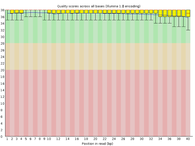
The x-axis displays the base position in the read, and the y-axis shows quality scores. In this example, the sample contains reads that are 40 bp long. This is much shorter than the reads we are working with in our workflow. For each position, there is a box-and-whisker plot showing the distribution of quality scores for all reads at that position. The horizontal red line indicates the median quality score and the yellow box shows the 1st to 3rd quartile range. This means that 50% of reads have a quality score that falls within the range of the yellow box at that position. The whiskers show the absolute range, which covers the lowest (0th quartile) to highest (4th quartile) values.
For each position in this sample, the quality values do not drop much lower than 32. This is a high quality score. The plot background is also color-coded to identify good (green), acceptable (yellow), and bad (red) quality scores.
Now let's take a look at a quality plot on the other end of the spectrum.
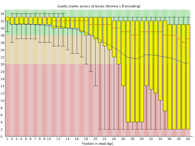
Here, we see positions within the read in which the boxes span a much wider range. Also, quality scores drop quite low into the "bad" range, particularly on the tail end of the reads. The FastQC tool produces several other diagnostic plots to assess sample quality, in addition to the one plotted above.
Running FastQC
We will now assess the quality of the reads that we downloaded. First, make sure you're still in the raw_data directory
cd ~/2020-NSURP/raw_data
Next, activate the conda environment we created in the Install Conda lesson.
conda activate nsurp-env
Now, use conda to install fastqc.
conda install fastqc
FastQC can accept multiple file names as input, and on both zipped and unzipped files, so we can use the *.fastq* wildcard to run FastQC on all of the FASTQ files in this directory.
fastqc *.fastq*
The FastQC program has created several new files within our directory.
For each input FASTQ file, FastQC has created a .zip file and a
.html file. The .zip file extension indicates that this is
actually a compressed set of multiple output files. We'll be working
with these output files soon. The .html file is a stable webpage
displaying the summary report for each of our samples.
Transferring data from Farm to your computer
To transfer a file from a remote server to our own machines, we will use scp.
To learn more about scp, see the bottom of this tutorial.
Now we can transfer our HTML files to our local computer using scp. The ./ indicates that you're transferring files to the directory you're currently working from.
scp -P 2022 -i /path/to/key/file username@farm.cse.ucdavis.edu:~/2020-NSURP/raw_data/*.html ./
If you're on a mac using zsh, you may need to replace the scp with noglob scp in the command above.
If you're on windows, you may need to move the the files from the download location on your Linux shell over to the windows side of your computer before opening.
Once the file is on your local computer, double click on it and it will open in your browser. You can now explore the FastQC output.
Decoding the FastQC Output
We've now looked at quite a few "Per base sequence quality" FastQC graphs, but there are nine other graphs that we haven't talked about! Below we have provided a brief overview of interpretations for each of these plots. For more information, please see the FastQC documentation here
- Per tile sequence quality: the machines that perform sequencing are divided into tiles. This plot displays patterns in base quality along these tiles. Consistently low scores are often found around the edges, but hot spots can also occur in the middle if an air bubble was introduced at some point during the run.
- Per sequence quality scores: a density plot of quality for all reads at all positions. This plot shows what quality scores are most common.
- Per base sequence content: plots the proportion of each base position over all of the reads. Typically, we expect to see each base roughly 25% of the time at each position, but this often fails at the beginning or end of the read due to quality or adapter content.
- Per sequence GC content: a density plot of average GC content in each of the reads.
- Per base N content: the percent of times that 'N' occurs at a position in all reads. If there is an increase at a particular position, this might indicate that something went wrong during sequencing.
- Sequence Length Distribution: the distribution of sequence lengths of all reads in the file. If the data is raw, there is often on sharp peak, however if the reads have been trimmed, there may be a distribution of shorter lengths.
- Sequence Duplication Levels: A distribution of duplicated sequences. In sequencing, we expect most reads to only occur once. If some sequences are occurring more than once, it might indicate enrichment bias (e.g. from PCR). If the samples are high coverage (or RNA-seq or amplicon), this might not be true.
- Overrepresented sequences: A list of sequences that occur more frequently than would be expected by chance.
- Adapter Content: a graph indicating where adapater sequences occur in the reads.
- K-mer Content: a graph showing any sequences which may show a positional bias within the reads.
Extra Info
if you ever need to download >10 accessions from the SRA, the sra-toolkit is a great tool to do this with!
However, we find sra-toolkit cumbersome when only a couple accessions need to be downloaded.