In [1]:
>>> %matplotlib inline
>>> from pylab import *
>>> import numpy
>>> import khmer, screed
Manipulating k-mer abundance spectra
Let’s turn to the question of k-mer abundances.
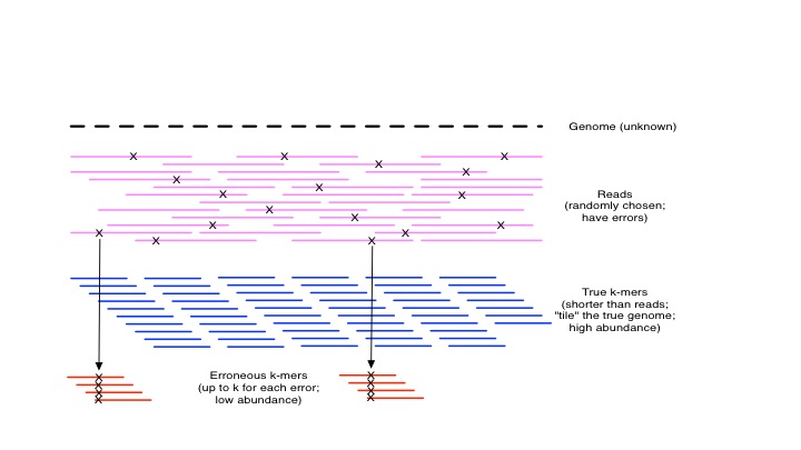
Suppose you have 200x coverage of a 1kb single-copy linear DNA sequence in 100 bp reads. On average, with truly random and uniform sampling, you would see every base in the true sequence 1000 times, with about half more frequently and half less frequently. You could measure this quite easily with mapping - simply map all the reads to the linear sequence, and then count the number of times each base is covered by a read.
In [2]:
>>> # !bowtie2-build data/genome.fa data/genome
>>> # !gunzip -c data/reads.fa.gz | bowtie2 data/genome -f -  > data/reads.map
>>> coverhist = numpy.loadtxt('data/reads.map.cover')
>>> plot(coverhist[:,0], coverhist[:,1])
Out[2]:
[<matplotlib.lines.Line2D at 0x10589e278>]

If, however, you don’t know the true sequence, you can still estimate the coverage by looking at the histogram of k-mer abundances, or k-mer abundance spectrum:
In [3]:
>>> !abundance-dist-single.py -q -k 21 -M 1e6 -s data/reads.fa.gz temp/hist.out
making countgraph
building k-mer tracking graph
kmer_size: 21
k-mer countgraph sizes: [227271, 227269, 227267, 227265]
outputting to temp/hist.out
consuming input, round 1 -- data/reads.fa.gz
Total number of unique k-mers: 246028
preparing hist from data/reads.fa.gz...
consuming input, round 2 -- data/reads.fa.gz
wrote to: temp/hist.out
In [4]:
>>> hist = numpy.loadtxt('temp/hist.out', skiprows=1, delimiter=',')
>>> plot(hist[:,0], hist[:,1])
>>> title('k-mer abundance histogram for data/reads.fa.gz')
>>> xlabel('k-mer abundance')
>>> ylabel('N k-mers with that abundance')
Out[4]:
<matplotlib.text.Text at 0x105955a20>

Here, there are two peaks: one is the peak of true k-mer abundances, which is around x=140. The other is the set of erroneous k-mers resulting from sequencing errors. The intuition is simple: in general, erroneous k-mers will only show up a few times, while k-mers that are generated from sampling true sequence will show up many times.
kmers
In [5]:
>>> plot(hist[:,0], hist[:,1])
>>> title('erroneous k-mers in data/reads.fa.gz')
>>> xlabel('k-mer abundance')
>>> ylabel('N k-mers with that abundance')
>>> axis(xmax=10)
Out[5]:
(0.0, 10, 0.0, 180000.0)

In [6]:
>>> plot(hist[:,0], hist[:,1])
>>> title('real k-mers in data/reads.fa.gz')
>>> xlabel('k-mer abundance')
>>> ylabel('N k-mers with that abundance')
>>> axis(ymax=500)
Out[6]:
(0.0, 180.0, 0.0, 500)

If we color the true k-mers blue and the erroneous k-mers red, this is quite clear:
In [7]:
>>> !load-into-counting.py -q -k 21 -M 1e6 temp/reads.kh data/reads.fa.gz

>>> !abundance-dist.py -q -s temp/reads.kh data/genome.fa.gz temp/hist-real.csv

>>> hist_real = numpy.loadtxt('temp/hist-real.csv', delimiter=',', skiprows=1)
>>> plot(hist_real[:,0], hist_real[:,1], 'r-', label='real k-mers')
>>> plot(hist[:,0], hist[:,1], 'b--', label='error k-mers')
>>> legend(loc='upper right')
>>> axis(ymax=500)
Saving k-mer countgraph to temp/reads.kh
Loading kmers from sequences in ['data/reads.fa.gz']
making countgraph
consuming input data/reads.fa.gz
Total number of unique k-mers: 249310
saving temp/reads.kh
fp rate estimated to be 0.179
DONE.
wrote to: temp/reads.kh.info
Counting graph from temp/reads.kh
K: 21
outputting to temp/hist-real.csv
** squashing existing file temp/hist-real.csv
preparing hist...
Out[7]:
(0.0, 180.0, 0.0, 500)

This is a nice demonstration of the “error catastrophe” of k-mer based views of sequencing data – in any reasonable sequencing data set, there are many more erroneous k-mers (area under the left curve) than there are real k-mers (area under the right curve).
This difference in abundance peaks lets us do error analysis and trimming.
Finding errors in reads
For example, errors can readily be identified in reads by looking at the first location where a low-abundance k-mer appears:
In [8]:
>>> first_read = next(iter(screed.open('data/reads.fa.gz')))
>>> first_seq = first_read.sequence

>>> cg = khmer.load_countgraph('temp/reads.kh')
>>> counts = cg.get_kmer_counts(first_seq)

>>> plot(range(len(counts)), cg.get_kmer_counts(first_seq))
>>> xlabel('position in read')
>>> ylabel('k-mer abundance at that position')
>>> title('k-mer abundance profile of the first read')
Out[8]:
<matplotlib.text.Text at 0x105daf198>

Trimming low-abundance k-mers
And, of course, you can simply remove all the low-abundance k-mers from reads altogether, leaving only the high-abundance k-mers:
In [9]:
>>> !filter-abund.py -q temp/reads.kh data/reads.fa.gz -C 5 -o temp/reads.trimmed.fa

>>> !abundance-dist-single.py -q -s -k 21 -M 1e6 temp/reads.trimmed.fa temp/trimmed.csv

>>> hist_trim = numpy.loadtxt('temp/trimmed.csv', delimiter=',', skiprows=1)
>>> plot(hist_trim[:,0], hist_trim[:,1], 'g*-', label='trimmed k-mers')

>>> plot(hist[:,0], hist[:,1], 'b--', label='error k-mers')
>>> plot(hist_real[:,0], hist_real[:,1], 'r-', label='real k-mers')
>>> legend(loc='upper right')
>>> axis(ymax=600)
loading countgraph: temp/reads.kh
K: 21
filtering data/reads.fa.gz
starting threads
starting writer
loading...
... filtering 0
done loading in sequences
DONE writing.
processed 20000 / wrote 16216 / removed 3784
processed 2000000 bp / wrote 1216425 bp / removed 783575 bp
discarded 39.2%
output in temp/reads.trimmed.fa
making countgraph
building k-mer tracking graph
kmer_size: 21
k-mer countgraph sizes: [227271, 227269, 227267, 227265]
outputting to temp/trimmed.csv
consuming input, round 1 -- temp/reads.trimmed.fa
Total number of unique k-mers: 10065
preparing hist from temp/reads.trimmed.fa...
consuming input, round 2 -- temp/reads.trimmed.fa
wrote to: temp/trimmed.csv
Out[9]:
(0.0, 180.0, 0.0, 600)

If you look at the k-mer abundance spectrum of the trimmed k-mers (green) against the abundance spectrum of the whole data set (red), you will see that in effect we’ve shifted the abundance spectrum left - this is because we are trimming reads at low-abundance k-mers and discarding the remainder of the reads, rather than simply ignoring the low abundance k-mers.
Error trimming decreases memory consumption
Error trimming has the advantage of dramatically simplifying several issues: first, you don’t have nearly as many k-mers to keep track of, which can decrease the total amount of memory needed to process the reads in another ways; and second, assembly itself becomes much simpler if you are dealing with only correct k-mers, because then only repeats are problematic.
On the flip side, as you can see above, you lose quite a bit of data - the abundance histogram shifts quite far left - because when you trim reads at low-abundance k-mers, you also trim off high-abundance data to the right of them. There are ways to deal with this loss of data but in practice with high coverage data sets it’s not a problem.
What else can we do with k-mer abundance spectra?
Variable coverage error trimming
The above approach of identifying low-abundance k-mers as errors works well in situations where you have high, uniform coverage of the molecules in your sample. This is possible to achieve with genomes by doing deep enough sequencing because the single copy sequence will be represented uniformly. But what about transcriptomes and metagenomes and MD-amplified samples? Any such samples of sufficient diversity will have both high-abundance components and low-abundance components.
For example, consider a two-species metagenome, where one species (species A) is present at 100x the abundance of the other. If we sequence species A to 1000x, species B will still only be present at 10x within the sample:
In [10]:
>>> !abundance-dist-single.py -s -q -M 1e7 data/mixed-reads.fa.gz temp/mixed-reads.hist

>>> mixed_hist = numpy.loadtxt('temp/mixed-reads.hist', skiprows=1, delimiter=',')
>>> plot(mixed_hist[:,0], mixed_hist[:,1])

>>> axis(ymax=1000)
>>> title('real k-mers in data/mixed-reads.fa.gz')
>>> xlabel('k-mer abundance')
>>> ylabel('N k-mers with that abundance')
making countgraph
building k-mer tracking graph
kmer_size: 32
k-mer countgraph sizes: [2272726, 2272724, 2272722, 2272720]
outputting to temp/mixed-reads.hist
consuming input, round 1 -- data/mixed-reads.fa.gz
Total number of unique k-mers: 87754
preparing hist from data/mixed-reads.fa.gz...
consuming input, round 2 -- data/mixed-reads.fa.gz
wrote to: temp/mixed-reads.hist
Out[10]:
<matplotlib.text.Text at 0x105be6668>

If we abundance trim at k-mers with abundance 3 as above, we’ll eliminate almost all of the real data from species B (the peak on the left), along with many of the errors in species A (the peak on the right, and the errors for which are in the peak on the left).
In [11]:
>>> !filter-abund-single.py -q -M 1e6 -k 21 -C 10 data/mixed-reads.fa.gz
>>> !mv mixed-reads.fa.gz.abundfilt temp/mixed-trim.fa

>>> !abundance-dist-single.py -q -s -M 1e6 -k 21 temp/mixed-trim.fa temp/mixed-trim.hist

>>> mixed_trim_hist = numpy.loadtxt('temp/mixed-trim.hist', skiprows=1, delimiter=',')
>>> plot(mixed_trim_hist[:,0], mixed_trim_hist[:,1])

>>> axis(ymax=1000)
>>> title('k-mers in data/mixed-trim-hist.fa.gz')
>>> xlabel('k-mer abundance')
>>> ylabel('N k-mers with that abundance')
making countgraph
consuming input, round 1 -- data/mixed-reads.fa.gz
Total number of unique k-mers: 70437
fp rate estimated to be 0.004
filtering data/mixed-reads.fa.gz
starting threads
starting writer
loading...
... filtering 0
done loading in sequences
DONE writing.
processed 5508 / wrote 4395 / removed 1113
processed 550800 bp / wrote 345804 bp / removed 204996 bp
discarded 37.2%
output in mixed-reads.fa.gz.abundfilt
making countgraph
building k-mer tracking graph
kmer_size: 21
k-mer countgraph sizes: [227271, 227269, 227267, 227265]
outputting to temp/mixed-trim.hist
consuming input, round 1 -- temp/mixed-trim.fa
Total number of unique k-mers: 5588
preparing hist from temp/mixed-trim.fa...
consuming input, round 2 -- temp/mixed-trim.fa
wrote to: temp/mixed-trim.hist
Out[11]:
<matplotlib.text.Text at 0x105d0a4e0>

Note that there’s an additional problem, too: deep sequencing of highly abundant molecules will yield erroneous k-mers with abundance > 3. We don’t really see that here but if we increased the coverage to 1000 we would.
What we need to do here is use a cutoff for error abundance that takes into account the local abundance of the read. While this may not be something that we know, we can estimate it on a per-read basis by looking at the other k-mers in the read – for example, if most of the k-mers in a read are high abundance in the overall data set, then probably the read itself is high abundance and any low-abundance k-mers in it are erroneous.
Practically speaking, we can guess the abundance of a read by using the median k-mer abundance of the k-mers in a read with respect to the overall k-mer spectrum. We can then choose our trimming cutoff so that k-mers outside the natural sampling spread of k-mers within the read are identified as errors:
In [12]:
>>> !load-into-counting.py -M 1e6 -k 21 -q temp/mixed-reads.kh data/mixed-reads.fa.gz
>>> !filter-abund.py -q -C 3 -V -Z 20 temp/mixed-reads.kh data/mixed-reads.fa.gz -o temp/mixed-trimV.fa

>>> !abundance-dist-single.py -q -s -M 1e6 -k 21 temp/mixed-trimV.fa temp/mixed-trimV.hist

>>> mixed_trimV_hist = numpy.loadtxt('temp/mixed-trimV.hist', skiprows=1, delimiter=',')
>>> plot(mixed_trimV_hist[:,0], mixed_trimV_hist[:,1], 'g-', label='variable coverage trimmed')

>>> mixed_trim_hist = numpy.loadtxt('temp/mixed-trim.hist', skiprows=1, delimiter=',')
>>> plot(mixed_trim_hist[:,0], mixed_trim_hist[:,1], 'b-', label='hard trimmed')

>>> legend(loc='upper right')
>>> axis(ymax=1000)
>>> xlabel('k-mer abundance')
>>> ylabel('N k-mers with that abundance')
Saving k-mer countgraph to temp/mixed-reads.kh
Loading kmers from sequences in ['data/mixed-reads.fa.gz']
making countgraph
consuming input data/mixed-reads.fa.gz
Total number of unique k-mers: 70437
saving temp/mixed-reads.kh
fp rate estimated to be 0.004
DONE.
wrote to: temp/mixed-reads.kh.info
loading countgraph: temp/mixed-reads.kh
K: 21
filtering data/mixed-reads.fa.gz
starting threads
starting writer
loading...
... filtering 0
done loading in sequences
DONE writing.
processed 5508 / wrote 4840 / removed 668
processed 550800 bp / wrote 403572 bp / removed 147228 bp
discarded 26.7%
output in temp/mixed-trimV.fa
making countgraph
building k-mer tracking graph
kmer_size: 21
k-mer countgraph sizes: [227271, 227269, 227267, 227265]
outputting to temp/mixed-trimV.hist
consuming input, round 1 -- temp/mixed-trimV.fa
Total number of unique k-mers: 21130
preparing hist from temp/mixed-trimV.fa...
consuming input, round 2 -- temp/mixed-trimV.fa
wrote to: temp/mixed-trimV.hist
Out[12]:
<matplotlib.text.Text at 0x105a80e48>

This has the effect of trimming off many errors for the high abundance reads, and trimming effectively no low-abundance reads. This is OK: it’s very hard to recover data you’ve eliminated, and for low-abundance reads, we must simply remain unsure of the distinction between “true” and erroneous k-mers.
(Underlying all of this, what we are really trying to do is estimate whether or not a k-mer belongs to one of two Poisson distributions: the “true k-mer” Poisson distribution, or the “erroneous k-mer” Poisson distribution. I am not aware of analytic solutions to this, but they might exist – they would be in Pevzner’s work on k-mer spectra from the early 2000s.)
Estimating per-read coverage, more generally
The ability to estimate a read’s coverage by looking at k-mer abundances is pretty handy, because you can do it without a reference, and therefore you can use it to extract reads from data sets without assembling
(You can’t use k-mer spectra alone to extract reads, because a read may have a mixture of high and low abundance k-mers in it.)
For example, in the situation above with two species, it is easy to extract all of the reads that belong to the high abundance species, species A – simply take any read with an estimated abundance greater than 50.
In [13]:
>>> import khmer.utils
>>> countgraph = khmer.load_countgraph('temp/mixed-reads.kh')

>>> fp = open('temp/mixed-high-abund.fa', 'wt')
>>> for record in screed.open('data/mixed-reads.fa.gz'):
...     if countgraph.get_median_count(record.sequence)[0] > 50:
...         khmer.utils.write_record(record, fp)
>>> fp.close()


>>> !abundance-dist-single.py -q -s -M 1e6 -k 21 temp/mixed-high-abund.fa temp/mixed-high-abund.hist

>>> mixed_high = numpy.loadtxt('temp/mixed-high-abund.hist', skiprows=1, delimiter=',')
>>> plot(mixed_high[:,0], mixed_high[:,1], 'r-', label='high coverage (estimated)')

>>> plot(mixed_trimV_hist[:,0], mixed_trimV_hist[:,1], 'g-', label='variable coverage trimmed')
>>> plot(mixed_trim_hist[:,0], mixed_trim_hist[:,1], 'b-', label='hard trimmed')

>>> legend(loc='upper right')
>>> axis(ymax=1000)
>>> xlabel('k-mer abundance')
>>> ylabel('N k-mers with that abundance')
making countgraph
building k-mer tracking graph
kmer_size: 21
k-mer countgraph sizes: [227271, 227269, 227267, 227265]
outputting to temp/mixed-high-abund.hist
consuming input, round 1 -- temp/mixed-high-abund.fa
Total number of unique k-mers: 54491
preparing hist from temp/mixed-high-abund.fa...
consuming input, round 2 -- temp/mixed-high-abund.fa
wrote to: temp/mixed-high-abund.hist
Out[13]:
<matplotlib.text.Text at 0x1062b72b0>

Note that here we are taking the high coverage untrimmed (red line) - the errors are still there (the bump near x=0), but now they can be gotten rid of quite easily now.
Normalizing read coverages
Let’s consider the situation above with two species A and B. A is kind of a problem – the bulk of the sequencing data is from A, and we don’t really need 100x (or 1000x) coverage to recover the true genome of A. Is there a way to get rid of some of those reads?
We could slice high coverage reads out, and then subsample the reads down to a coverage of 50x or so; or, we can do something else that turns out to be effectively the same thing, but is more efficient - read coverage normalization, or “digital normalization” in khmer parlance.
In [14]:
>>> !normalize-by-median.py -q -C 20 -k 21 -M 1e6 data/mixed-reads.fa.gz -o temp/mixed-norm.fa

>>> !abundance-dist-single.py -q -s -M 1e6 -k 21 temp/mixed-norm.fa temp/mixed-norm.hist

>>> mixed_norm = numpy.loadtxt('temp/mixed-norm.hist', skiprows=1, delimiter=',')
>>> plot(mixed_norm[:,0], mixed_norm[:,1], 'r-', label='normalized data')

>>> legend(loc='upper right')
>>> axis(ymax=1000)
>>> xlabel('k-mer abundance')
>>> ylabel('N k-mers with that abundance')
making countgraph
building k-mer tracking graph
kmer_size: 21
k-mer countgraph sizes: [227271, 227269, 227267, 227265]
outputting to temp/mixed-norm.hist
consuming input, round 1 -- temp/mixed-norm.fa
Total number of unique k-mers: 40385
preparing hist from temp/mixed-norm.fa...
consuming input, round 2 -- temp/mixed-norm.fa
wrote to: temp/mixed-norm.hist
Out[14]:
<matplotlib.text.Text at 0x106442dd8>

What digital normalization is doing is splitting the data in two - into reads with novel information, and redundant reads.
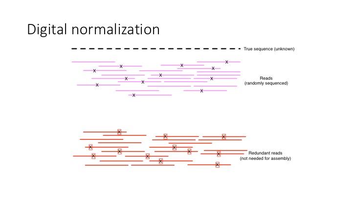
digital normalization
It also has the effect of reducing the error content of data all on its own – because we are discarding reads, we are also discarding errors in those reads.
We don’t have a good formal analysis of digital normalization, but the basic algorithm is:
for read in dataset:
   if estimated_coverage(read) < C:
      keep(read)
where estimated_coverage is the median k-mer abundance estimator,
above. This algorithm is:
- online
- streaming
- sublinear memory
Semi-streaming
Digital normalization points the way towards another interesting idea, which is that if you can detect when incoming reads have reached high coverage, you can start making decisions as the data comes in. This is explored in a preprint, Zhang et al., 2014; the basic idea is pictured below.
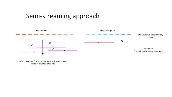
semi streaming
We have software that uses the semi-streaming approach to trim reads - so, like filter-abund.py above, but without the need to count all the k-mers first:
In [15]:
>>> !trim-low-abund.py -q -M 1e6 -C 3 -V -Z 20 data/mixed-reads.fa.gz -o temp/mixed-trimV-2.fa

>>> !abundance-dist-single.py -q -s -M 1e6 -k 21 temp/mixed-trimV-2.fa temp/mixed-trimV-2.hist

>>> mixed_trimV_hist = numpy.loadtxt('temp/mixed-trimV-2.hist', skiprows=1, delimiter=',')
>>> plot(mixed_trimV_hist[:,0], mixed_trimV_hist[:,1], 'g-', label='variable coverage trimmed (streaming)')

>>> mixed_trim_hist = numpy.loadtxt('temp/mixed-trim.hist', skiprows=1, delimiter=',')
>>> plot(mixed_trim_hist[:,0], mixed_trim_hist[:,1], 'b-', label='hard trimmed')

>>> legend(loc='upper right')
>>> axis(ymax=1000)
>>> xlabel('k-mer abundance')
>>> ylabel('N k-mers with that abundance')
making countgraph
created temporary directory ./tmpno0p49odkhmer; use -T to change location
data/mixed-reads.fa.gz: kept aside 2780 of 5508 from first pass, in data/mixed-reads.fa.gz
second pass: looking at sequences kept aside in ./tmpno0p49odkhmer/mixed-reads.fa.gz.pass2
removing ./tmpno0p49odkhmer/mixed-reads.fa.gz.pass2
removing temp directory & contents (./tmpno0p49odkhmer)
read 5508 reads, 550800 bp
wrote 4652 reads, 415196 bp
looked at 2780 reads twice (1.50 passes)
removed 856 reads and trimmed 1413 reads (41.19%)
trimmed or removed 24.62% of bases (135604 total)
5508 reads were high coverage (100.00%);
skipped 0 reads/0 bases because of low coverage
fp rate estimated to be 0.001
output in *.abundtrim
making countgraph
building k-mer tracking graph
kmer_size: 21
k-mer countgraph sizes: [227271, 227269, 227267, 227265]
outputting to temp/mixed-trimV-2.hist
consuming input, round 1 -- temp/mixed-trimV-2.fa
Total number of unique k-mers: 30227
preparing hist from temp/mixed-trimV-2.fa...
consuming input, round 2 -- temp/mixed-trimV-2.fa
wrote to: temp/mixed-trimV-2.hist
Out[15]:
<matplotlib.text.Text at 0x10662d588>

Perhaps one of the biggest missing pieces of khmer is the lack of a formal presentation and analysis of these ideas. Maybe we’ll write something up this fall :).
Is the true sequence still present?
With all of these manipulations to remove errors and redundancy in sequencing data sets, it is always nice to check that our beginning principle holds true - that the k-mers of the true genomic sequence remain in the data set.
A simple way to do that (in simulated data) is to use the abundance histogram functionality to look to see how many true k-mers are present in the read data set.
We don’t have a script to do this, but we can do the reverse - below, we ask how many of the true k-mers are missing from the final data set:
In [16]:
>>> !load-into-counting.py -q -k 21 -M 1e7 data/mixed-trimV2.fa.kh temp/mixed-trimV-2.fa

>>> !abundance-dist.py -q -s data/mixed-trimV2.fa.kh data/mixed-species.fa.gz temp/mixed-trimV-2.x.species.hist
>>> !head -2 temp/mixed-trimV-2.x.species.hist
Saving k-mer countgraph to data/mixed-trimV2.fa.kh
Loading kmers from sequences in ['temp/mixed-trimV-2.fa']
making countgraph
consuming input temp/mixed-trimV-2.fa
Total number of unique k-mers: 30229
saving data/mixed-trimV2.fa.kh
fp rate estimated to be 0.000
DONE.
wrote to: data/mixed-trimV2.fa.kh.info
Counting graph from data/mixed-trimV2.fa.kh
K: 21
outputting to temp/mixed-trimV-2.x.species.hist
** squashing existing file temp/mixed-trimV-2.x.species.hist
preparing hist...
abundance,count,cumulative,cumulative_fraction
0,20,20,0.002
...and the answer is, 0.2%, which is pretty good.
K-mer abundance histograms are a powerful way to look at & manipulate short read data sets, but they are only one way. Next, we will look at graph-based approaches.
Next: Exploring graphs